
Switch Join: PostgreSQL that adapts on the fly
Adaptive join algorithm in Postgres.


PostgreSQL’s query optimizer (and most others) struggles with cardinality misestimation that leads to the choice of a suboptimal plan. Switch Join provides runtime adaptivity to PostgreSQL’s execution pipeline, allowing the engine to combine join strategies in a single execution node on the fly.
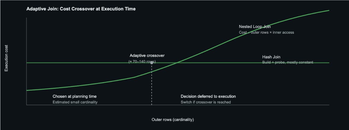
Switch Join covers two equivalent join strategies upfront: an optimistic “as is” plan (usually Nested Loop) and a pessimistic backup plan (typically Hash or Merge Join). Execution starts with the optimistic plan while materializing outer tuples. It watches the actual outer row count, and when it exceeds a threshold, Switch Join changes its strategy to a pessimistic one. Without restarting the execution of a backup plan from scratch, it rescans the already materialized outer tuples and continues working.
I would like to share my experience of creating such a complex yet fascinating project, which my colleague A. Lepikhov and I developed together, as well as explain the core concept on which the PostgreSQL extension with an adaptive join was built. Unfortunately, we cannot provide the source code publicly - only a Docker container is available.
In addition, I presented this technology at PGConf.Dev 2025 (Montreal, Canada) in a talk titled “Switching between query plans in real time (Switch Join)” and at PostgreSQL IvorySQL EcoConference (HOW) 2025 in a talk titled “PostgreSQL Optimizer Flaws: Real Stories and How We Fix Them”, and decided to write an article about it.
This article explains how the approach works, discusses implementation details, and shows the performance improvements we observed.
The problem: when optimizers guess wrong
The process of finding an optimal plan is complex and primarily based on selectivity estimation (the proportion of rows (cardinality) in the result relative to the maximum possible) and cardinality. Based on cardinality estimates, not only is the order of relation pair combinations selected to ensure that fewer rows are processed in subsequent joins, but also the cost, that is, the expense measured in PostgreSQL’s special units for executing an operation or algorithm.
There are three possible join algorithms: Nested Loop, Hash Join, and Merge Join. More details can be found here. Thus, underestimation or overestimation leads to uncertainty in finding the optimal query plan.
Cardinality calculation is based on statistics, as is cost calculation for algorithms. Regarding algorithms, for example, for hash joins, the uniqueness of the relation selected for building the hash table is evaluated to understand collision risks. Query planning in PostgreSQL is a cost-based model, and basically follows the logic: the cheaper the algorithm, the better it is. It tries to throw away the worst plan candidates in the early stage of the planning, which have a higher cost. More information about this can be found here.
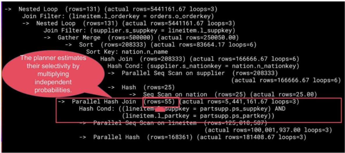
There are a lot of reasons why the optimizer predicts cardinality incorrectly and, as a result, generates a suboptimal query plan that leads to longer execution. Statistics may be inaccurate due to infrequent updates or limited sampling. Another common cause is column correlation: the simplified assumption of independence used in prediction often leads to incorrect cardinality estimation. The articles below provide many examples of this topic, where such cases are discussed in detail.
Leis et al. How Good Are Query Optimizers, Really? (VLDB 2015) demonstrated that cardinality estimates in major databases can be off by factors up to 10⁶, with compounding errors across joins.
Robert Haas. Query Planning Gone Wrong (PostgreSQL Conference) perhaps best summarizes the issue with a relatable quote.
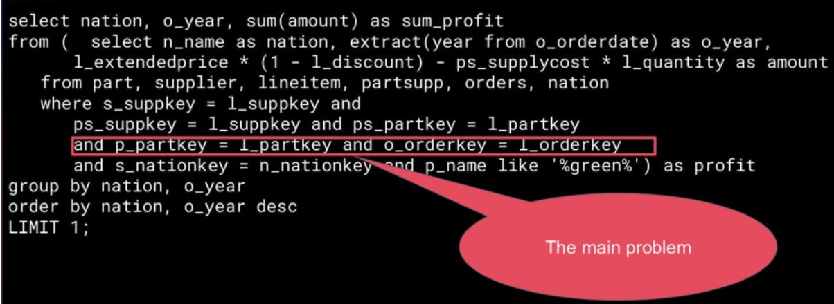
Other scenarios observed in the TPC-H benchmark include query 9.sql, where columns represent the same entity, and this information is not taken into account during prediction without using extended statistics.
Here is the 9.sql query:
                            QUERY PLAN
-----------------------------------------------------------------
 GroupAggregate  (cost=872.57..872.62 rows=5 width=48) (actual time=1800000.000..1800000.000 rows=25 loops=1)
   ->  Nested Loop  (cost=0.57..872.57 rows=444 width=44) (actual time=0.610..1800000.000 rows=16000000 loops=1)
         ->  Nested Loop  (cost=0.29..80.72 rows=2221 width=36) (actual time=0.039..334.000 rows=8000 loops=1)
               ->  Seq Scan on part  (cost=0.00..58.71 rows=20 width=20) (actual time=0.014..0.315 rows=8000 loops=1)
                     Filter: (p_name ~~ '%green%'::text)
               ->  Index Scan using partsupp_pkey on partsupp  (cost=0.29..1.10 rows=111 width=16) (actual time=0.002..0.002 rows=2000 loops=8000)
                     Index Cond: ((ps_partkey = part.p_partkey) AND (ps_suppkey = supplier.s_suppkey))
         ->  Index Scan using lineitem_pkey on lineitem  (cost=0.29..0.36 rows=1 width=28) (actual time=0.002..0.002 rows=2000 loops=8000)
               Index Cond: ((l_partkey = partsupp.ps_partkey) AND (l_suppkey = partsupp.ps_suppkey))

 Planning Time: 1.041 ms
 Execution Time: 1800000.000 ms
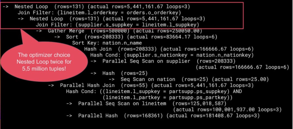
The PostgreSQL optimizer treats the fields `ps_suppkey` and `ps_partkey` as independent when estimating selectivity. In reality, they form a strongly correlated pair — together they identify a single tuple in the `partsupp` table, which is a composite key. Because of this statistical independence assumption, the optimizer grossly underestimates how many rows will survive the joins and chooses Nested Loop as the best option.
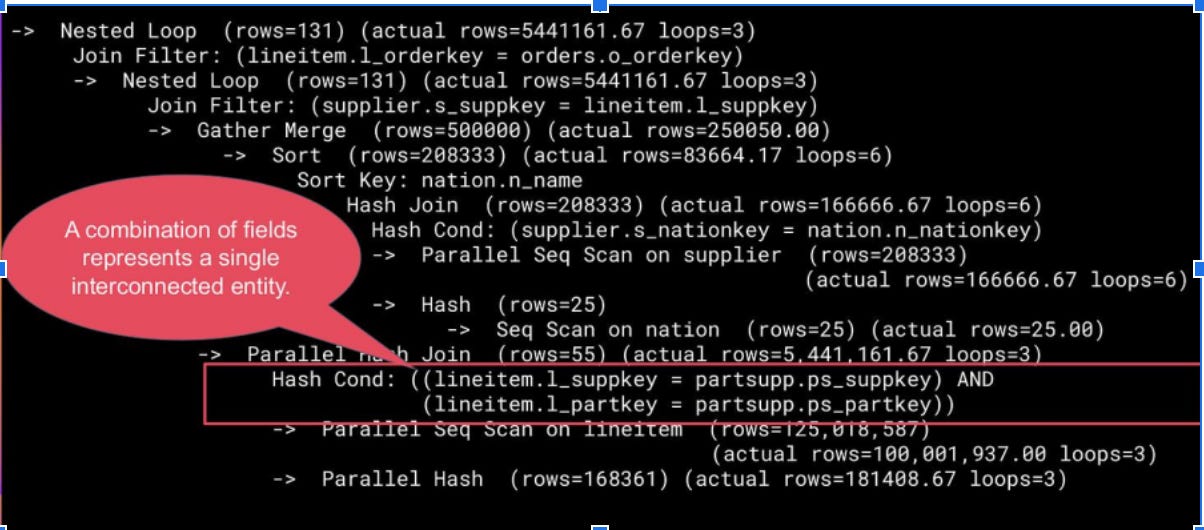
With extended statistics (Distinct) for l_suppkey, l_partkey, and ps_suppkey, ps_partkey, the cardinality estimation can’t be fixed, but it pushes the optimizer to generate an optimal plan with Hash Join:
                               QUERY PLAN
------------------------------------------------------------------------
 GroupAggregate  (cost=108.48..289.73 rows=444 width=48) (actual time=234.250..234.255 rows=25 loops=1)
   ->  Hash Join  (cost=108.48..289.73 rows=444 width=44) (actual time=231.245..234.250 rows=16000000 loops=1)
         Hash Cond: (lineitem.l_partkey = partsupp.ps_partkey AND lineitem.l_suppkey = partsupp.ps_suppkey)
         ->  Hash Join  (cost=80.72..180.21 rows=2221 width=36) (actual time=0.656..2.426 rows=16000000 loops=1)
               Hash Cond: (partsupp.ps_partkey = part.p_partkey AND partsupp.ps_suppkey = supplier.s_suppkey)
               ->  Seq Scan on part  (cost=0.00..58.71 rows=20 width=20) (actual time=0.014..0.315 rows=8000 loops=1)
                     Filter: (p_name ~~ '%green%'::text)
               ->  Hash  (cost=80.72..80.72 rows=2221 width=16) (actual time=0.624..0.624 rows=8000000 loops=1)
                     Buckets: 262144  Batches: 32  Memory Usage: 2048kB
                     ->  Seq Scan on partsupp  (cost=0.00..80.72 rows=2221 width=16) (actual time=0.006..0.697 rows=8000000 loops=1)
         ->  Hash  (cost=155.00..155.00 rows=10000 width=28) (actual time=230.589..230.589 rows=6000000 loops=1)
               Buckets: 262144  Batches: 32  Memory Usage: 2048kB
               ->  Seq Scan on lineitem  (cost=0.00..155.00 rows=10000 width=28) (actual time=0.006..0.633 rows=6000000 loops=1)

 Planning Time: 43.892 ms
 Execution Time: 379425.591 ms
Switch Join helps here too and constructs two versions of the plan: the original Nested Loop chosen by the optimizer (Plan A — "as Is"), and a backup Hash Join designed for large cardinalities (Plan B — “Pessimistic”). As the query runs, Switch Join monitors the row count flowing through the outer relation of the Nested Loop and, after preserving them with the Materialize node, it rescans them instead of recomputing and switches to the Hash Join node.
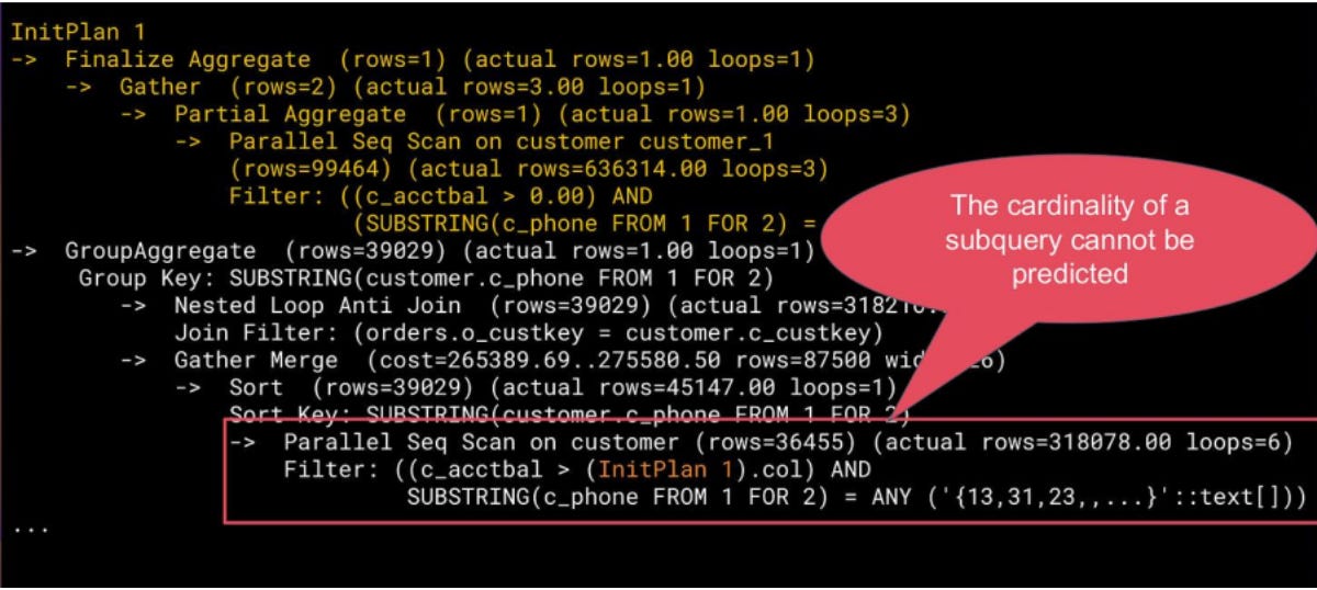
Another example is query 22.sql, where it is impossible to predict the result of a subquery in advance, and without rewriting the query, there is no way to solve this problem.
Here is the 22.sql query:
SELECT cntrycode, COUNT(*) AS numcust, SUM(c_acctbal) AS totacctbal
FROM (
SELECT SUBSTRING(c_phone FROM 1 FOR 2) AS cntrycode, c_acctbal
FROM customer
WHERE SUBSTRING(c_phone FROM 1 FOR 2) IN ('13','31','23','29','30','18','17')
AND c_acctbal > (
SELECT AVG(c_acctbal)
FROM customer
WHERE c_acctbal > 0.00
AND SUBSTRING(c_phone FROM 1 FOR 2) IN ('13','31','23','29','30','18','17'))
AND NOT EXISTS (
SELECT * FROM orders WHERE o_custkey = c_custkey)
) AS custsale
GROUP BY cntrycode
ORDER BY cntrycode;
QUERY PLAN
------------------------------------------------------------------------
GroupAggregate (cost=125.50..150.75 rows=7 width=20) (actual time=1800000.000..1800000.000 rows=7 loops=1)
-> Nested Loop (cost=0.57..124.76 rows=4 width=16) (actual time=0.053..1800000.000 rows=45000 loops=1)
Join Filter: (NOT (SubPlan 1))
-> Seq Scan on customer (cost=0.00..58.71 rows=20 width=16) (actual time=0.032..91.160 rows=45000 loops=1)
Filter: ((substring((c_phone)::text, 1, 2) = ANY ('{13,31,23,29,30,18,17}'::text[])) AND (c_acctbal > (SubPlan 2)))
-> Index Scan using orders_o_custkey_idx on orders (cost=0.29..3.30 rows=1 width=4) (actual time=0.002..0.002 rows=0 loops=45000)
Index Cond: (o_custkey = customer.c_custkey)
Planning Time: 7.454 ms
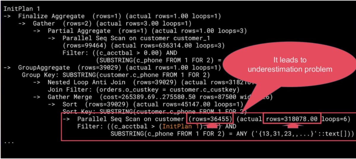
Execution Time: 1800000.000 msThe problem lies in the query’s structure: it contains an `InitPlan`, a separate subquery whose cardinality is almost impossible to predict before execution. Because the optimizer doesn’t calculate `InitPlans` before planning the outer query, its estimate is wildly off. The planner sees what appears to be a small result set and chooses a Nested Loop join strategy.
Switch Join addresses this by deferring the decision between nested loop and hash join until execution. It starts with the optimizer's chosen plan (typically Nested Loop) while materializing outer tuples and monitoring the actual row count. When the threshold is exceeded, Switch Join switches mid-query to a Hash Join strategy.
The competitive landscape
Over the years, developers have tried various approaches: improving predictions, learning from past mistakes, or replanning mid-query. Each has its trade-offs. Switch Join does something different: it adapts at runtime without replanning.
Introduced in PostgreSQL 10, Extended Statistics help the optimizer predict correlations better, which improves selectivity and cardinality estimates and fixes some of the raised problems earlier. But sometimes it is not a suitable solution. While `ANALYZE` updates extended statistics, the fundamental problem remains: there is no automatic creation of extended statistics, and it requires a complicated and time-consuming analysis. As data distributions change, some column combinations may no longer need extended statistics, while others that previously didn’t require them now do. Besides, we have limited resources for creating extended statistics. It needs not only memory to store them, but also ANALYZE will need them to be updated constantly, which leads to extra workload for the system.
PostgreSQL’s O. Ivanov, S. Bartunov. Adaptive Cardinality Estimation for PostgreSQL (2017) extension was one of the first in-house attempts to address persistent cardinality misestimations. AQO collects runtime feedback from executed queries and uses it to refine future cardinality estimates. It effectively shares with the planner actual cardinality information of nodes that it stores during the plan generation process when the user runs this query again.
The benefit is straightforward: the planner no longer relies solely on static statistics. Instead, it incorporates observed row counts from past executions to improve subsequent plans.
The limitation is equally clear. AQO is fundamentally reactive. Like extended statistics, it depends on historical feedback. As data distributions shift, this feedback can become stale, gradually reducing its reliability.
Another approach introduced in PostgresPro Enterprise: Adaptive Query Execution, also known as Realtime Query Replanning. It is similar to AQO: it also keeps cardinality statistics up to date and shares them with the optimizer during planning. However, instead of waiting for the query to be manually executed by the user, it automatically triggers replanning and uses the information collected at the previous stage. This process continues until an optimal plan is found and the trigger no longer fires, or until further plan optimization becomes impossible.
The primary benefit of query replanning is correctness under severe misestimation due to data skew, correlation, or rapidly changing distributions based on actual runtime observations.
This method improves accuracy but comes at a cost — higher computational overhead.
A Generalized Join Algorithm (Goetz Graefe, HP Labs) proposed a single adaptive join operator that could emulate Nested Loop, Hash Join, or Merge Join, and switch between them at runtime. Instead of committing to a Join strategy during planning, the operator adapts based on observed cardinalities, available memory, and data ordering during execution.
The key advantage is flexibility. If memory pressure increases or data skew becomes apparent, the operator can spill, re-hash, or re-sequence data without restarting the query or invoking a full replanning phase.
However, this generality comes at a significant implementation cost. Join algorithms differ not only in execution mechanics, but also in their parameterization and access patterns. Nested Loop and Merge Join often rely on efficient index usage compared to Hash Join, ordering guarantees, and plan-time decisions about outer/inner roles. These properties are difficult to abstract and adjust dynamically at runtime.
All these techniques have the same problem: they either need pre-execution corrections (like extended stats and AQO) or full replanning (like Realtime Replanning). Switch Join works differently: it adapts at runtime without replanning.
The missing piece: Adaptive or Switch Join
This technology is not a new concept, and many companies have attempted to implement it.
Amazon Aurora’s Adaptive Join addresses cardinality misestimation using a runtime switching mechanism, but its execution strategy and threshold calculation method differ fundamentally from Switch Join, which will be observed later.
Aurora starts execution with the optimizer’s chosen plan, usually a Nested Loop join, and monitors the actual row count from the outer side. If it exceeds a precomputed crossover threshold (the point where a Hash Join becomes cheaper), Aurora switches strategies. It builds a hash table and restarts the join using a Hash Join.
The threshold is derived during planning via cost-based analysis of Nested Loop and Hash Join, scaled by a configurable multiplier:
crossover_threshold = estimated_rows×apg_adaptive_join_crossover_multiplier
Microsoft Adaptive Join takes a different approach from both Aurora. Unlike these systems that switch from Nested Loop to Hash Join, Microsoft Adaptive Join operates in the opposite direction: it starts with a Hash Join and switches to Nested Loop if the actual row count is smaller than a threshold. This “pessimistic-first” strategy assumes that the join will be large and prepares the hash table upfront. If the actual input turns out to be small (below the threshold), Microsoft Adaptive Join abandons the hash table and switches to a Nested Loop join. This approach is particularly useful when the optimizer overestimates the cardinality, as it can quickly adapt to the smaller actual size without wasting resources on hash table construction for small joins.
Switch Join follows an optimistic approach, starting with the optimizer’s chosen plan (typically a Nested Loop join) and monitoring the actual row count during execution. As tuples flow through the outer relation, Switch Join materializes them to reuse later. If the actual row count exceeds a predefined threshold, Switch Join switches to a Hash Join using the already materialized outer tuples, avoiding repeated scans of the outer relation. This runtime adaptation occurs without query replanning, allowing the system to correct optimizer mistakes on the fly. The detailed architecture, execution flow, and switching mechanism are discussed in depth in the sections below.
Optimistic vs. pessimistic: which way to switch?
This raises a fundamental question: does it make sense to consider both approaches simultaneously? The two strategies operate from fundamentally different philosophical starting points. Microsoft Adaptive Join follows a pessimistic approach: execution begins with a Hash Join, essentially assuming from the start that there will be an error in cardinality estimation. In contrast, Switch Join follows an optimistic approach: it assumes that cardinality was predicted correctly and starts with the optimizer’s chosen plan (typically Nested Loop).
Both concepts make sense, but in different scenarios. The pessimistic approach (starting with Hash Join) shines when there’s a high probability of cardinality errors. Consider cases with GROUP BY operations downstream that can dramatically alter row counts, or known patterns where statistics consistently fail. In scenarios where the cost of a wrong Nested Loop far exceeds the cost of an unnecessary hash table, paying upfront makes sense.
The optimistic approach (starting with Nested Loop), however, finds its strength in uncertainty. Sometimes statistics can be inaccurate, and we can’t always predict when. This might happen under a high write load, before VACUUM has updated the statistics, or on large tables where sampling coverage is insufficient. Even so, we still have to rely on them. By starting optimistically and adapting on the fly, we avoid unnecessary overhead in most cases. The overhead of early hash table construction would be wasteful when statistics are generally reliable, even if occasionally stale.
The overhead and process also differ fundamentally between the two approaches. In the pessimistic case (Microsoft Adaptive Join), they immediately build the hash table. It’s expensive if there are actually few tuples or if the planner didn’t err in its estimate. In the optimistic case (Switch Join), the overhead is on materialization, but it occurs only during the switch. Switch Join is more efficient when estimates are accurate, but potentially slower to react when estimates are wrong from the start.
But these are questions to ponder. Now, let’s take a closer look at what Switch Join is and how it works.
Demonstration of the problem on simple case
To demonstrate the problem, let’s reproduce it with the simplest case.
DROP TABLE IF EXISTS a,b CASCADE;

CREATE TABLE a WITH (autovacuum_enabled = false) AS SELECT gs % 10 AS x, gs as y FROM generate_series(1,1E1) AS gs;

CREATE TABLE b WITH (autovacuum_enabled = false) AS SELECT gs AS x FROM generate_series(1,1E1) AS gs; -- It is the easiest way to emulate optimizer error ...

ANALYZE a,b;

INSERT INTO a SELECT gs%5 AS gs, gs%5 as y FROM generate_series(1,1E6) AS gs;
INSERT INTO b SELECT 1 AS x FROM generate_series(1,1E3) AS gs;

SELECT count(*) FROM a, b WHERE a.x = b.x AND a.y = 2;
Observed planner behavior and execution outcome:
The planner underestimates the join size (thinks ~1 row) and picks a Nested Loop.
Reality: ~200k qualifying rows from a, each probing b → 200,001 passes over b.
Result: ~22.5 s runtime (looping itself into oblivion).
				QUERY PLAN
------------------------------------------------------------------------
 Aggregate  (rows=1) (actual time=22503.042..22503.043 rows=1 loops=1)
   ->  Nested Loop  (rows=1) (actual time=0.053..22489.535 rows=200001 loops=1)
         Join Filter: (a.x = b.x)
         Rows Removed by Join Filter: 201801009
         ->  Seq Scan on a  (rows=1) (actual time=0.032..91.160 rows=200001 loops=1)
               Filter: (y = '2'::numeric)
               Rows Removed by Filter: 800009
         ->  Seq Scan on b  (rows=50) (actual time=0.002..0.040 rows=1010 loops=200001)

 Planning Time: 7.454 ms
 Execution Time: 22503.106 ms
(10 rows)
With Switch Join (runtime humility)
Switch Join execution behavior and outcome:
Two plans are prepared: As-is (Nested Loop) and Pessimistic (Hash Join).
Execution starts with Nested Loop, counts outer rows, hits the tiny switch threshold (10), then switches to Hash Join.
                 	   Query Plan
------------------------------------------------------------------------
 Aggregate  (rows=1) (rows=1 loops=1)
    ->  Custom Scan (SwitchJoin)  (rows=1) (rows=200001 loops=1)
    --> Limit cardinality: 10
        ->  Nested Loop  (never executed)
              Join Filter: (a.x = b.x)
              ->  Materialize  (rows=510 loops=2)
                    ->  Seq Scan on b  (rows=510 loops=2)
              ->  Materialize  (never executed)
                    ->  Seq Scan on a  (never executed)
                          Filter: (y = ‘2’::numeric)
        ->  Hash Join  (rows=1) (rows=200001 loops=1)
              Hash Cond: (a.x = b.x)
              ->  Seq Scan on a  (rows=1) (rows=200001 loops=1)
                    Filter: (y = ‘2’::numeric)
                    Rows Removed by Filter: 800009
              ->  Hash  (rows=50) (rows=1010 loops=1)
                    Buckets: 1024  Batches: 1  Memory Usage: 45kB
                    ->  Materialize  (rows=50) (rows=510 loops=2)
                          ->  Seq Scan on b  (rows=50) (rows=510 loops=2)

 Planning Time: 0.229 ms
 Execution Time: 120.102 ms
 (21 rows)
Enter Switch Join: planning two worlds
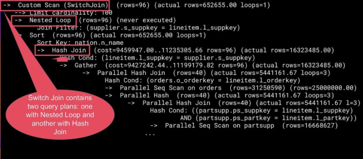
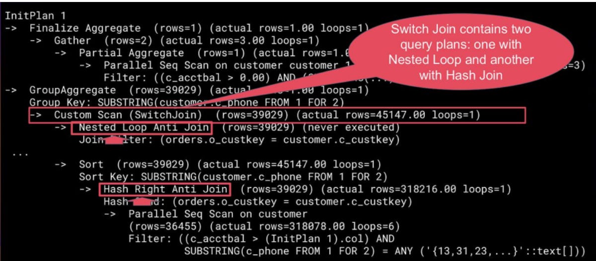
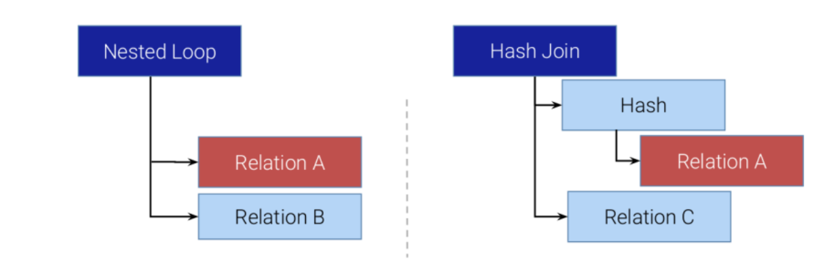
Switch Join introduces a dual-plan execution model. During planning, it constructs two complete versions of the same query fragment:
“As-Is” plan is the optimizer’s original vision, assuming its estimates are correct. Typically, this means choosing a fast, index-driven Nested Loop join for “small” results.
A pessimistic plan is a safeguard plan built under the assumption that the optimizer’s cardinality prediction is wrong (specifically, that it underestimates). This alternative usually prefers a Hash or Merge Join, which scales better for large result sets.
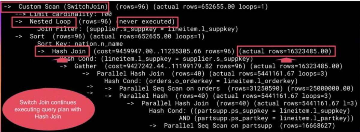
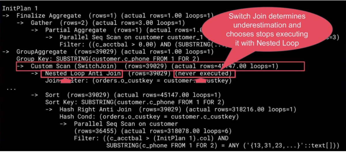
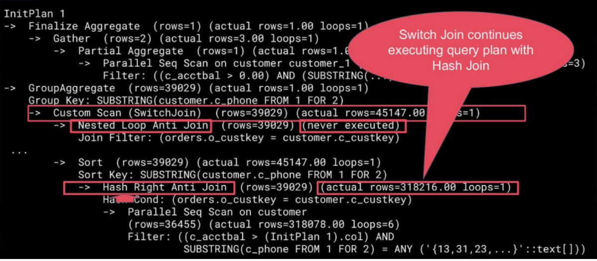
Both plans are preserved in the executor. The magic happens during runtime: as PostgreSQL starts reading tuples from the outer relation, Switch Join observes the actual row count. If it surpasses a predefined threshold, the extension dynamically switches to the pessimistic plan mid-execution.
This way, the planner doesn’t have to be omniscient. It just needs to prepare a backup plan for when its optimism proves misplaced.
You can understand it through analogy.

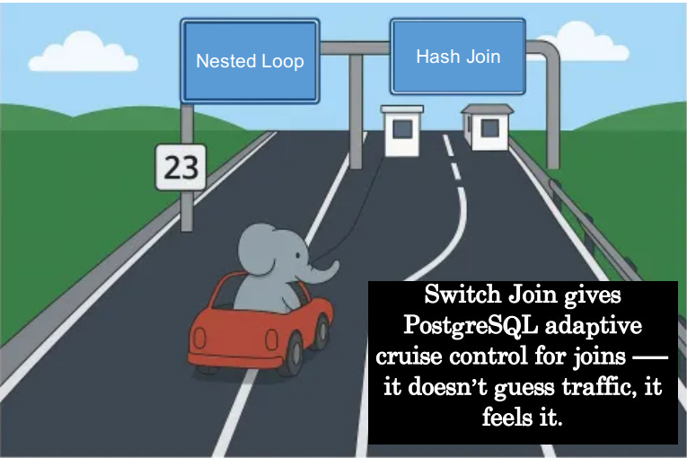
Imagine PostgreSQL as a little elephant driving down a data highway toward a toll plaza — two lanes ahead:
🟢 Manual Lane: fast, efficient, but only if traffic is light.
⚡ Express Lane built for heavy traffic: slower to start but faster when the line gets long.
When our elephant (the query executor) starts its journey, it doesn’t yet know how heavy traffic will be. If it guesses wrong and takes the manual lane during rush hour, it’ll be stuck behind a thousand cars, honking in pain (a Nested Loop with millions of rows). If it always takes the express lane, it wastes time paying extra tolls when traffic is almost empty (unnecessary Hash Join setup).
So, what does Switch Join do? It installs a traffic sensor right before the toll booths — a smart counter that measures how many cars (tuples) are ahead.
If the road looks clear, the elephant cruises through the Manual Lane (Nested Loop). But if the traffic piles up, he uses Express Lane (Hash Join).
This analogy mirrors the exact logic under the hood:
The traffic sensor = runtime row counter.
The manual lane = Nested Loop (great for small datasets).
The express lane = Hash Join (ideal for large datasets).
The lane switch = dynamic plan replacement once the row count threshold is exceeded.
How the switching works
Switch Join runs the “as-is” plan while materializing outer results in a shared buffer and watching row counts. Once a threshold is exceeded, it switches mid-query to the pessimistic Hash or Merge Join, no replanning or restart needed. It’s built with lightweight, modular Custom Nodes and tunable heuristics, so the switch is safe, efficient, and fully adaptive.
The execution flow
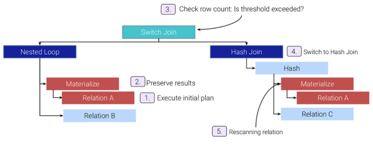
Here’s how it works:
Execute the initial plan. PostgreSQL starts with the “as-is” Nested Loop plan.
Preserve results. The output from the outer node is materialized to avoid recomputation.
Monitor cardinality. A counter tracks how many rows have been processed so far.
Threshold check. When the row count exceeds the switching limit (defined via cost-based heuristics or GUCs), the system triggers a switch.
Rescan and continue. Execution transitions to the pessimistic Hash Join or Merge Join plan, using the preserved data as input.
This switch happens without replanning, locking, or restarting the query. It’s a mid-execution fix for the optimizer misstep.
The internal architecture: building Switch Join
Switch Join is built entirely with PostgreSQL Custom Nodes, so it plugs directly into the planner and executor without changing core files.
Only a single hook is used: set_rel_pathlist_hook, ensuring the extension remains modular and non-invasive.
Path preparation
Both plans use the same outer path to ensure they produce the same results and avoid recomputation. We need this because recomputing the outer side could give inconsistent results or waste time.
This setup ensures that when switching occurs, PostgreSQL doesn’t re-read data — it simply continues execution using the materialized buffer.
Materialization
The materialized node is shared between both Join strategies. The Nested Loop consumes tuples normally, while the Hash Join can build its hash table from the same buffer. To maintain correctness, volatile or side-effect-producing functions are forbidden as outer inputs (e.g., random(), generate_series(), or CTEs with updates), since their re-evaluation could produce inconsistent results.
Setting the threshold: when to switch
The threshold determining when to switch from Nested Loop to Hash Join can be different:
Fixed: e.g., always switch after 1,000 outer rows.
Relative: multiply the estimated cardinality by a mistrust factor.
threshold = MIN(MAX(mistrust_factor × estimated_rows, min_limit, max_limit))
Heuristic: adjust dynamically based on join type, cost ratios, or observed data skew, or based on a cost model like it was built in AuroraDB.
Ultimately, we choose the relative method.
These parameters are tunable through GUCs:
switch_join.mistrust_factor — defines distrust in the optimizer’s estimate (1, 2, 10, …).
switch_join.min_limit_cardinality and max_limit_cardinality — boundaries for min and max cardinalities.
In benchmarks, a mistrust_factor of 2.5 offered the best balance between sensitivity and overhead.
Nested Loops: from bottleneck to adaptivity
Nested Loops work well for small or highly selective joins, but when the outer relation is underestimated, it leads to repeated scans and quadratic runtime. Switch Join preserves the initial Nested Loop plan for small datasets but dynamically switches to Hash or Merge Join when row counts grow unexpectedly. This allows queries to scale efficiently when cardinality is misestimated.
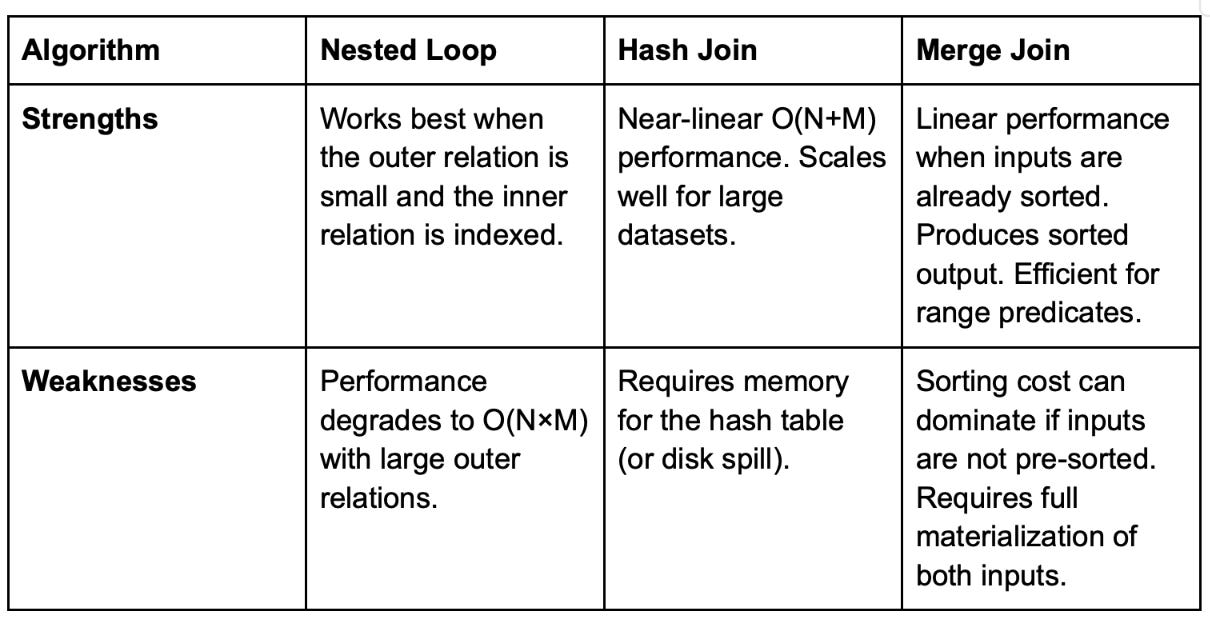
Brief overview: join algorithms
Before diving into the algorithms, remember that every join in PostgreSQL involves two inputs:
Outer relation → the table (or subquery) scanned first. Its rows drive the join process.
Inner relation → the table scanned for each outer row (or block of rows), typically using a join condition like a.x = b.x.

Philosophy of Nested Loop replacement
Before we consider the logic of replacement, Nested Loop with Switch Join, let’s break down the variants of Nested Loop and delve into its advantages and flaws.
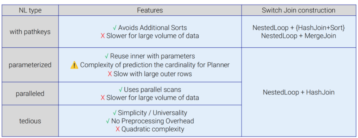
Classic Nested Loop (with PathKeys)
Nested Loop joins reuse data ordering provided by indexes, preserving pathkeys and allowing operations like ORDER BY or GROUP BY to avoid explicit sorting. This makes them highly efficient for small inputs or queries with very selective predicates. However, their performance degrades catastrophically as input sizes grow. Due to quadratic behavior, each row from the outer relation triggers a separate index lookup on the inner side, making Nested Loop joins impractical for large result sets.
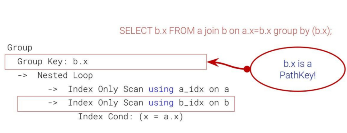
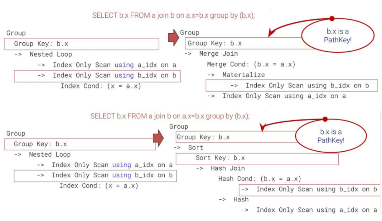
Switch Join allows a Nested Loop join to be dynamically replaced by either a Hash Join with a subsequent Sort, or by a Merge Join, depending on what is cheaper.
Parameterized Nested Loop
The inner relation depends on a parameter from the outer row, which makes execution efficient if the outer relation is small and index lookups are highly selective. However, the planner struggles to estimate cardinality accurately because parameterized filters can expand dramatically depending on data correlation. In such cases, each outer row may trigger thousands of repeated index scans.
Switch Join addresses this by dynamically replacing the Nested Loop with a Hash Join, reducing repeated work and improving performance.
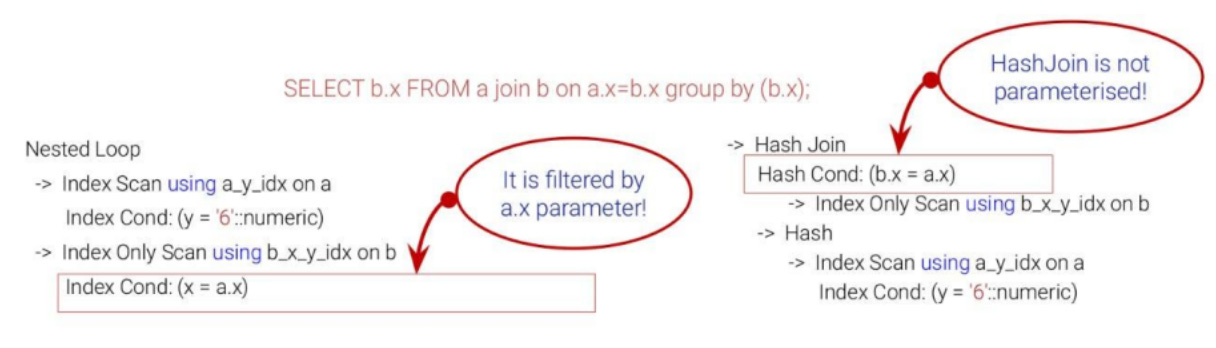
A critical concern is preserving parameterized Nested Loops rather than replacing them with Switch Join. While flushing a trivial Nested Loop may be acceptable, flushing a parameterized Nested Loop (PNL) is problematic. Since we have not yet fully resolved parameterization issues and param_info is initialized, add_path will remove PNLs from the pathlist along with trivial NLs if we’re not careful. We want to avoid this because parameterized paths serve a specific purpose: they enable efficient index lookups when the inner relation depends on parameters from the outer row. Therefore, when dealing with parameterized Nested Loops, we preserve both the PNL and the Switch Join in the pathlist, allowing the planner to choose the most appropriate path based on the query context.
And we have a question here. Since we have two paths — often a parameterized Nested Loop and a non-parameterized Hash Join — we may get different row counts at the output of each node. This raises another important question: if we are not parameterized from above, should we return the same number of tuples? To preserve semantics and avoid breaking query correctness, we maintain the order of tuples and add a rescan operation when switching between paths. This ensures that the output remains consistent regardless of which path is active, but it represents an open area for further investigation and optimization.
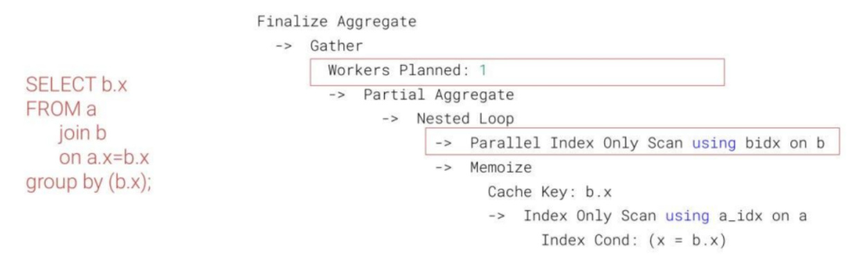
Parallel Nested Loop
Parallel Nested Loop leverages parallel-aware outer scans to utilize multiple CPU cores. While this improves throughput on small or moderately sized inputs, it still suffers from underestimation. When the outer relation is large, each worker may perform repeated full scans, and the overhead of parallel execution amplifies the cost of misestimation.
In Switch Join, the Nested Loop is replaced by an appropriate Hash Join with disabled parallelism. This design choice stems from the complexity of safely materializing scanned tuples for each worker and the difficulty of safely interrupting a Nested Loop mid-execution — challenges that make a parallel adaptive join impractical.
Basic (sequential) Nested Loop is simple but inflexible, scanning both relations linearly. It is typically chosen when no indexes exist or when the planner estimates a low cost. Its main drawback is quadratic runtime on large datasets, and the planner can stubbornly stick to it even when indexes are present, but statistics are misleading.
Switch Join addresses this by replacing the Nested Loop with a Hash Join, improving performance on larger or misestimated inputs.
The challenges of Nested Loops replacement
When deciding whether to preserve a Nested Loop or replace it with Switch Join, several fundamental questions arise that shape our implementation approach. These are the core questions we faced during development:
How should Switch Join paths be ranked against each other? Can we remove an old Switch Join if a more optimal one is found (e.g., in terms of the backup Hash Join)?
Should we allow only a single Switch Join in the pathlist, modifying it if a more optimal NL/HJ pair is found?
These questions represent fundamental design decisions that impact both the complexity of the implementation and the quality of the resulting query plans. To address these challenges while maintaining implementation simplicity, we developed a simplified approach:
Protect the first found Nested Loop (the cheapest one).
Generate our own Hash Join rather than looking at Hash Joins from the pathlist.
This approach reduces complexity while still providing the core adaptive behavior.
To understand the specific challenges, we need to understand the context of how Switch Join paths are inserted into PostgreSQL’s planning infrastructure. The pathlist represents a list of alternative paths, sorted by total_cost. It may contain paths of various types (for a join relation, not only NestPath, HashPath, or MergePath) and also already contain a Switch Join path inserted in a previous iteration.
With this context in mind, the implementation faces several challenges that we addressed:
Preserving existing paths. We must not flush existing paths from the pathlist, as they may be better than ours, especially since we do not support all modes — parallel queries or parameterized path chains, for example. The goal is to add Switch Join as an option, not to replace all existing paths.
Suboptimal Switch Join combinations. Switch Join can be highly suboptimal if not carefully constructed. For instance, a poor Nested Loop may be protected by switching to Hash Join, but we need to find the best Hash Join to switch to.
Combinatorial explosion. Switch Join paths should not noticeably expand the plan search space. Each potential replacement creates additional paths that the planner must consider, which could slow down planning time if not managed carefully.
Partial selection (LIMIT). We may select a suboptimal variant in queries with LIMIT clauses, where the optimizer’s choice of Nested Loop might actually be correct for the limited result set, even if cardinality estimates are wrong for the full dataset.
When inserting Switch Join paths into the planner’s pathlist, we must:
Find or generate a suitable path pair: Identify appropriate Nested Loop and Hash Join paths, or generate them if needed.
Work with copies: For paths already in the pathlist, create copies and operate on those copies to avoid modifying existing paths.
Insert via add_path: it helps us to avoid combinatorial explosion because it slways rejects suboptimal paths.
These challenges highlight that replacing Nested Loops with Switch Join is not simply a matter of swapping algorithms, but requires careful consideration of path selection, cost estimation, and integration with PostgreSQL’s existing planning infrastructure.
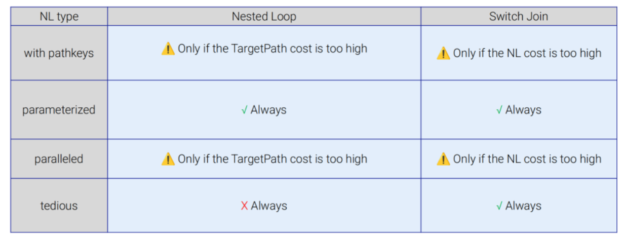
When using Switch Join instead of a standard Nested Loop, the system always replaces the conventional Nested Loop while preserving pathkeys. Parallel execution is enabled only if the planner estimates it to be cost-effective. For parameterized Nested Loops, both the original and target paths are retained, allowing the optimizer to defer the final choice based on the next generated path and runtime conditions.
Separately, I would like to discuss about the cost model of Switch Join that we implemented to ensure a path enters the pathlist without flushing the Nested Loop (including parameterized ones). We add cost model tuning for safe insertion and make total_cost slightly larger while setting startup_cost slightly smaller. This positions the Switch Join path just ahead of the specific Nested Loop, minimizing impact to only one path in the list. However, there may be some fluctuation, as other paths could fall into the gap between our Switch Join cost and the replaced Nested Loop. This cost manipulation is particularly important when dealing with parameterized paths, as it allows both the PNL and the Switch Join to coexist in the pathlist.
Testing results on TPC-H benchmarks
We put Switch Join to the test using the TPC-H benchmark — a standard workload designed by the Transaction Processing Performance Council to torture query optimizers with 22 complex analytical queries.
Each query operates on multi-gigabyte tables (lineitem, orders, supplier, customer, etc.), with deeply nested joins and correlated subqueries - a perfect storm for cardinality misestimation.
In this environment, even a single incorrect join order can turn a 5-second query into a 30-minute timeout.
The full testing results are available at https://github.com/Alena0704/TPC-H-test.
The bar chart shows absolute execution times for TPC-H queries with and without Switch Join (log scale).
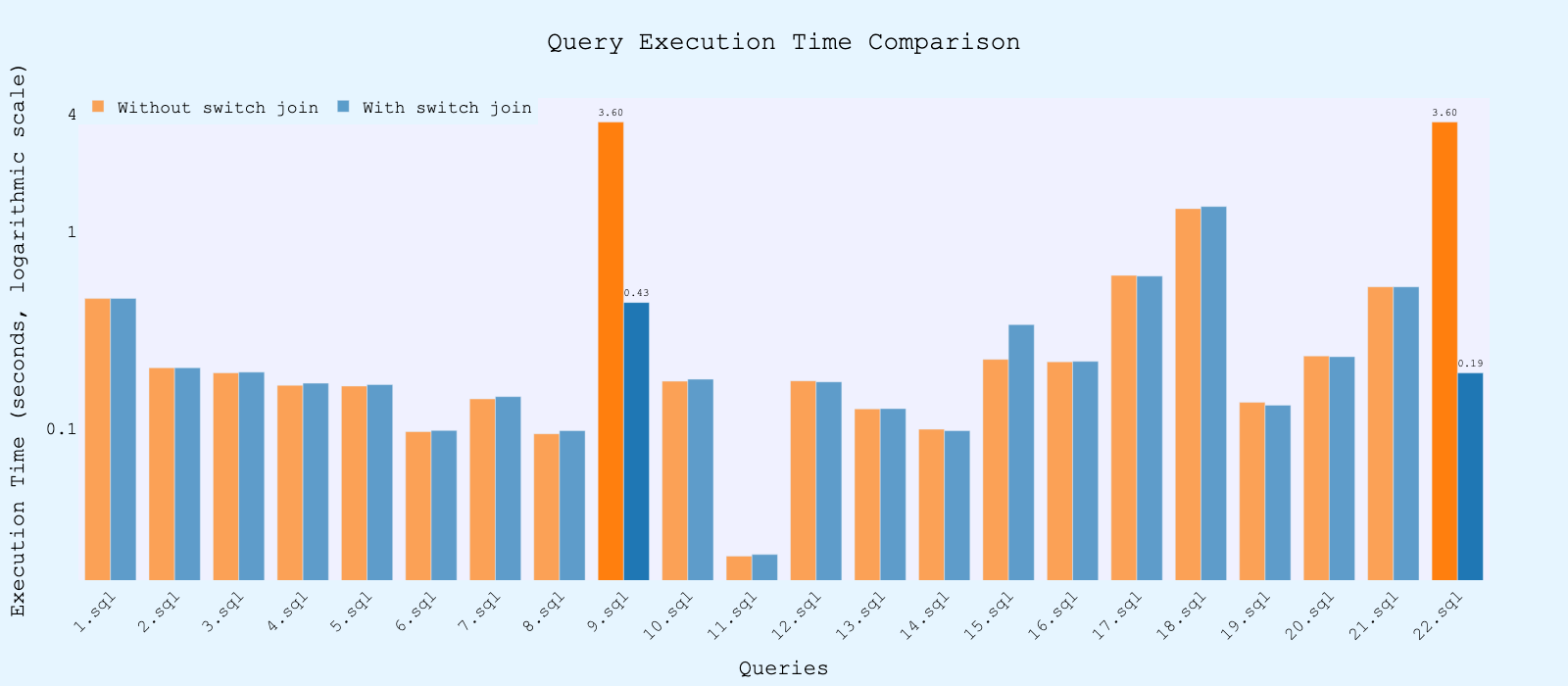
For most queries, performance remained neutral. This indicates that Switch Join introduces virtually no overhead - the adaptive mechanism is simply not triggered.
However, several queries show a dramatic difference. In particular, Q9 and Q22 perform extremely poorly without Switch Join, reaching the statement_timeout limit (≈1800 seconds). When Switch Join is enabled, execution time drops sharply:
Q9 completes in ~434 seconds
Q22 completes in ~190 seconds
Conclusion
Switch Join provides PostgreSQL with something it’s long been missing — the ability to adapt during query execution. Rather than committing to a plan based on imperfect guesses, it observes actual row counts and adapts mid-execution. It doesn’t prevent optimizer mistakes, but it makes them manageable and non-catastrophic.
In production environments, where stability and predictability of execution time are critically important, Switch Join addresses one of the most pressing issues - preventing long-running queries that cause timeouts, lock resources, and degrade overall system performance. When cardinality is misestimated - due to data skew, stale statistics, or unexpected correlations - a Nested Loop can turn a join that the planner considered “small” into a multi-minute or even multi-hour execution. With Switch Join, such scenarios are detected and corrected on the fly, ensuring fast and stable query execution even under conditions of uncertainty.
You can try Switch Join for yourself using the Docker container `alena0704/switch_join` on PostgreSQL 17.
In some references from your talks, not shown in the article, I see you mention SQL Server 2017 as previous implementation of Adaptive Joins.
The idea was first implemented by Oracle in 2013 with Oracle Database 12c:
https://oracleapex.com/ords/features/r/dbfeatures/features?feature_id=344
There's also a patent for it: https://patents.google.com/patent/US20140095472A1/en
If you plan presenting the project again, could you acknowledge that? 😇